Principles of Congestion Control

The Causes and Costs of Congestion

Scenario 1: Two Senders, a Router with Infinite buffers

• This scenario is where two separate computers (sender 1 and sender 2, above) are sending data over the network, and their paths overlap at one specific middle point (a single router or cable, called a “hop”).
• Imagine our two senders pump new data into the network at the exact same speed (λ_in¹​ bytes per second).
  • In this scenario, the network uses a bare-bones protocol. It sends packets once and never retries, slows down, or checks for lost data.
  • Both hosts funnel their traffic through one middle router connected to a single output line that can only handle a max speed of R.
  • This middle router has buffers that allow it to store incoming packets when the packet-arrival exceeds the outgoing link’s capacity. For now, we’ll assume that the router has an infinite amount of buffer space.

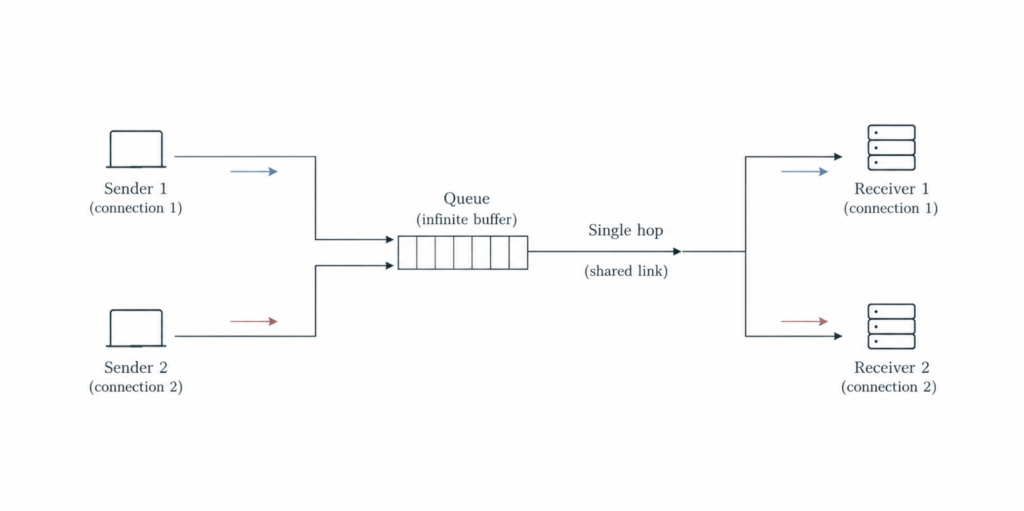
• The graphs below show what happens to Throughput (data delivered) and Delay (time spent waiting) as sender 1 increases its sending speed:

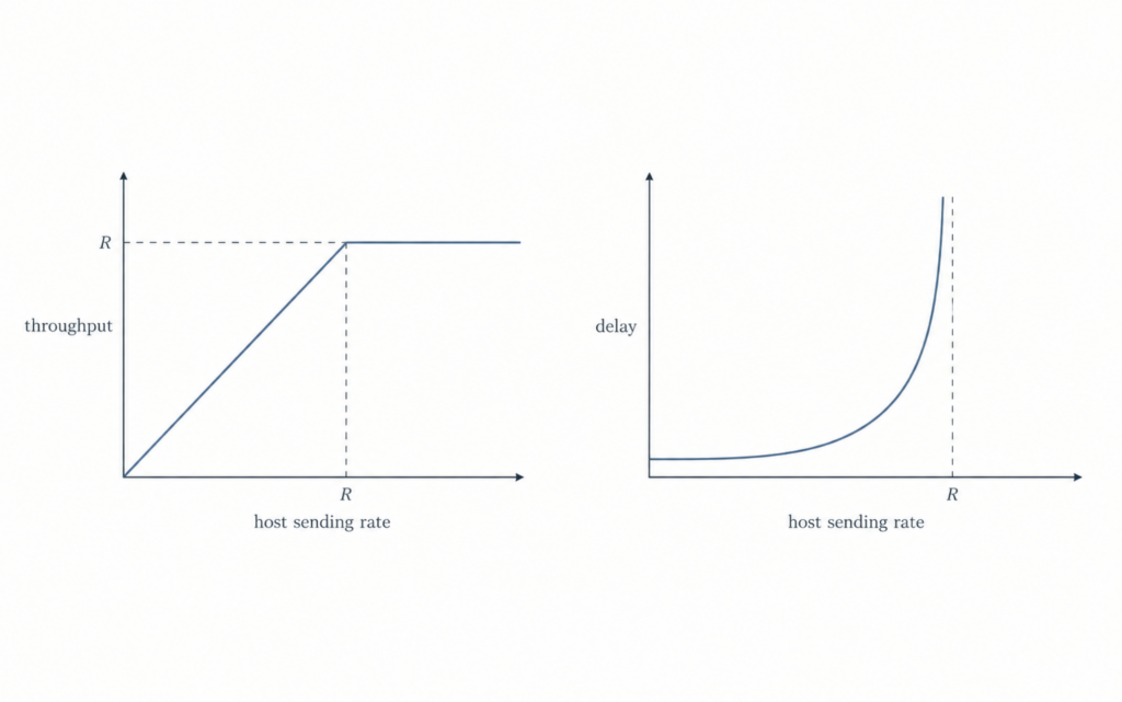
1. Graph 1: Throughput
   • Since the middle link has a max speed of R and is split equally between sender 1 and sender 2, sender 1’s personal limit is R/2.
   • If sender 1’s sending speed is between 0 and R/2, then everything they send gets delivered.
   • But if there sending speed is above R/2, then throughput hits a brick wall at R/2, If they try to send at 1000 Mbps, the pipe physically can only clear R/2, so pushing harder gives you zero extra speed.
2. Graph 2: Delay
   • As sender 1’s speed gets close to R/2, packets start arriving faster than the router can clear them. They sit in the router’s memory, so delay shoots up.
   • Because the buffer in this scenario is “infinite”, the line of waiting packets grows forever, causing infinite delay.

Scenario 2: Two Senders and a Router with Finite Buffers

• Now let’s assume the amount of router buffering is assumed to be finite.
  • The consequence of this is that packets will be dropped when arriving to an already full buffer.
• Let’s also assume that each connection is reliable i.e. if a packet is dropped at the router, the sender will eventually retransmit it.
  • Because lost packets have to be sent again, we now have to track two different sending speeds:
    1. λ_in (original data rate): the speed at which your application generates brand-new data.
    2. λ’_in (offered load): the total speed of everything pushed onto the network, which includes brand-new data PLUS retransmitted data packets.

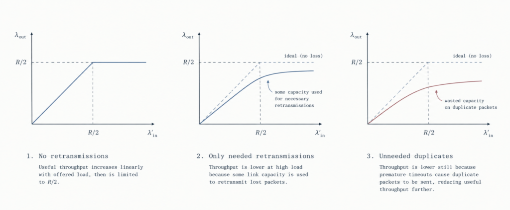
No retransmissions (graph 1, below):

• Let’s imagine a magical, hypothetical scenario where the sender has psychic powers and knows the exact state of the router.
  • In this scenario, host 1 would only send a packet if it knows for a fact that the router has an empty slot in its buffer. if the buffer is full, host 1 simply waits.
  • Because packets are only send where there is guaranteed space, the router never drops a single packet.
  • Since no packets are dropped, the sender never has to re-send old data (i.e. there’s zero retransmission). So every byte sent into the network is brand-new data (λ_in = λ’_in), and everything gets delivered on the first try.
• But, even with perfect efficiency, host 1 still cannot exceed a sending rate of R/2 because the shared output line physically cannot handle more than that.

Only needed retransmissions (graph 2, below):

• Now imagine a slightly more realistic scenario where the sender retransmits only when a packet is known for certain to be lost.
  • Again, this assumption is a bit of a stretch because it can’t be 100% sure about this, but the sending host might set its timer long enough to be virtually assured that a packet has been lost.
• So in this setup routers drop packets when their memory fills up, and senders retransmit only when a packet is guaranteed to be lost.
• Imagine pushing a total speed (λ’_in – the rate of original data transmission plus retransmission) of R/2 into the network.
  • The actual new data that successfully reaches the destination will obviously be less than R/2, because there’s going to be some water capacity spent resending packets that were dropped.
  • For example, you might push 0.5R worth of traffic, but 1/3 of that total effort is wasted just cleaning up past mistakes.
• The cost of a congested network, then, is that the sender must perform retransmissions in order to compensate for dropped (lost) packets due to buffer overflow.

Unneeded duplicates (graph 3, below):

• Finally, imagine the case that the sender may time out prematurely and retransmit a packet that has been delayed in the queue but not yet lost i.e. the sender gets impatient and resends a packet that is just stuck in traffic.
  • Here a packet get stuck waiting in a long router queue because the network is crowded
  • The sender’s time runs out (premature timeout) and thinks, therefore, the packet is lost. So sends a second copy.
  • Both the original packet and the duplicate copy eventually make it to the receiver.
  • The receiver keeps the first copy and throws the duplicate straight into the bin
• Here the router wasted time, energy, and link capacity carrying a duplicate packet that ended up in the bin – space that could’ve been used to deliver someone else’s actual data.

Scenario 3: Four Senders, Routers with Finite Buffers, and Multihop Paths

• In this final congestion scenario, the traffic traveling through multiple routers (hops) instead of just one.
• For instance, below we can see that for Host A to send data to Host C, it must pass through two consecutive routers (R1 and R2).
• Also, Host A doesn’t have these two routers (R1 and R2) to itself. It must share them. R1 is shared with data traveling from Host D to Host B. And R2 is shared with data traveling from Host B to Host D.

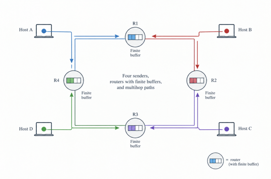
• When all computers are sending data at very low speeds (λ_in), the routers have plenty of extra memory, meaning dropped packets (buffer overflows) are rare.
  • Because packets aren’t being lost to full buffers, the amount of data successfully delivered to the destination essentially equals the amount of data pushed into the network i.e. throughput approximately equals the offered load
  • If the hosts increase their sending speeds slightly, throughput also goes up smoothly because the network still has leftover capacity to absorb the extra data without overflowing i.e. when λ_in is small, increases in λ_in result in an increase in λ_out

---

• Now let’s examine what happens if the multi-hop network is pushed to the absolute limit by putting loads of data into it (i.e. λ (and λ′ ) is extremely large.
  • Host A’s traffic (traveling to C) passes through R1 and then to R2. This traffic can have a maximum arrival rate at R2 that is never more than the capacity of the link from R1 to R2 (R).
  • Meanwhile, cross-traffic from Host B (travelling to D) may also be going through R2, which competes for the limited amount of buffer space.
  • Because Host B’s traffic does not have to pass through a prior bottleneck, its arrival rate at Router 2 can be much larger than Host A’s traffic. As the network becomes severely overloaded, Host B’s massive flood of packets instantly swallows up any empty slots in R2’s buffer.
  • As a result, the amount of Host A’s traffic that successfully survives Router 2 becomes smaller and smaller, eventually dropping to absolute zero (i.e A’s end-to-end throughput drops to 0).
• This creates a devastating chain reaction known as congestion collapse.
  • Every time Router 2 drops one of Host A’s packets, all the transmission capacity that Router 1 used to move that packet across the first hop is completely wasted.
  • The network burned through valuable upstream bandwidth to move a packet that was doomed at the second hop – capacity that could have been used to deliver a different packet successfully.

• Because of the severe penalties of uncontrolled traffic – like massive delays, wasted retransmissions, and total network collapse – networks desperately need a way to control how fast computers send data i.e. we need congestion control
• To solve this, network engineers focus on managing a connection’s bottleneck link.
  • When data travels from its source to its destination, the bottleneck is the specific link along the path that will choke on traffic first if senders try to speed up.

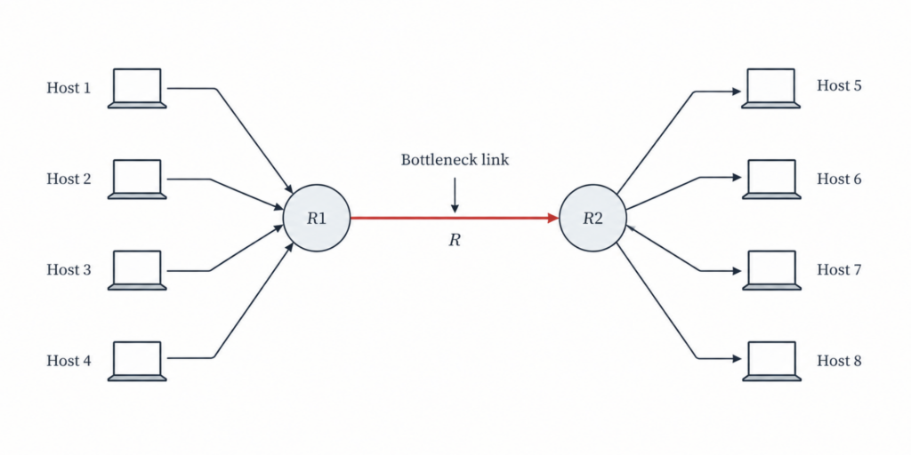
• When a group of separate connections (a total number we will call N) all force their data through the exact same bottleneck, that link quickly hits its absolute physical speed limit (capacity R).
  • If senders try to push data even faster, the bottleneck link physically cannot handle the extra load, meaning overall throughput will not increase
  • If the bottleneck shares its capacity fairly, its total speed limit (R) is split evenly among all N connections
  • As a result, the absolute maximum speed any single connection can achieve is R/N
• The purpose of congestion control is to find the perfect “Goldilocks” speed for all connections sharing a path.
  • If the total sending rate is lower than the bottleneck’s capacity, the link sits idle and wastes potential speed when there is still data waiting to be sent.
  • If the total sending rate exceeds the bottleneck’s capacity, it triggers all the severe congestion penalties, like dropped packets and massive delays.
  • So we’re trying to find a sending rate that’s “just right”. The combined speed of all senders should get as close as possible to the bottleneck’s maximum capacity without actually crossing it
• Two questions therefore come to mind:
  1. How does a connection know that a link on its source-to-destination path is congested, i.e. that there is a bottleneck link?
  2. How do connections individually regulate their sending rates so that their aggregate sending rate is close to, but does not exceed, their path’s bottleneck link capacity?

Approaches to Congestion Control

End-to-end Congestion Control

• With end-to-end congestion control, the network layer provides no explicit support to the transport layer for congestion-control purposes.
• The network layer doesn’t even tell the end systems there’s congestion (they simply have to infer congestion from observation e.g. packet loss and delay.
• TCP takes this end-to-end approach to congestion control.

Network-assisted Congestion Control

• With network-assisted congestion control, routers provide explicit feedback to the sender and/or receiver regarding the congestion state of the network.
• This feedback may be as simple as a single bit indicating congestion at a link.
• For example, in ATM Available Bite Rate (ABR) congestion control, a router informs the sender of the maximum host sending rate it (the router) can support on an outgoing link

1. λ_in​ (pronounced “lambda-in”) is simply the sending speed of the application – the rate at which a computer pumps brand-new data into the network. It’s usually measured in bytes per second (bytes/sec). ↩︎